Some mechanical concepts#
In this section, we will (depending on your background) define / repeat a few mechanical concepts. These are independent of the EMI model – simply useful mechanical quantities in general, some especially interesting in the cardiac setting.
Displacement and deformation#
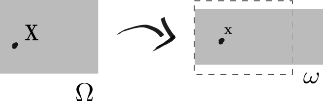
Reference configuration and current configuration. The reference domain \(\Omega\) is mapped to a new configuration \(\omega\), referred to as the current (deformed) configuration. Every point \(\mathbf{X} \in \Omega\) is mapped to a point \(\mathbf{x} \in \omega\).
We let \(\Omega\) be a three-dimensional domain. \(\Omega\) can be deformed to a new domain \(\omega\), the current or deformed configuration. Here every point \(\mathbf{X} \in \Omega\) is mapped to a new point \(\mathbf{x} \in \omega\). The displacement \(\mathbf{u}\), describing the difference between the new and the original position, can then be defined as
which is a vector. In the mechanical models utilized in this thesis, the displacement \(\mathbf{u}\) will usually be (one of) the unknowns which we solve for. Displacement can, however, also be more directly measured using image analysis techniques, simply by measuring the change in movement at given points between two different configurations.
From the displacement vector, we can define the deformation gradient:
where \(\mathbf{I}\) is the identity tensor. For the three-dimensional case, if the displacement is given by \(\mathbf{u} = (u_1, u_2, u_3)\) and any given point \(\mathbf{X} = (X_1, X_2, X_3)\), \(\mathbf{F}\) can be written out on matrix form as
The components are scalar functions which, unless the deformation is completely homogeneous, all have spatial distributions.
The Jacobian determinant \(J\) is defined based on the deformation tensor, defined by
which gives us the volume change of the material. If \(J = 1\), the volume is the same in the current as in the reference configuration.
The concepts of stress and strain#
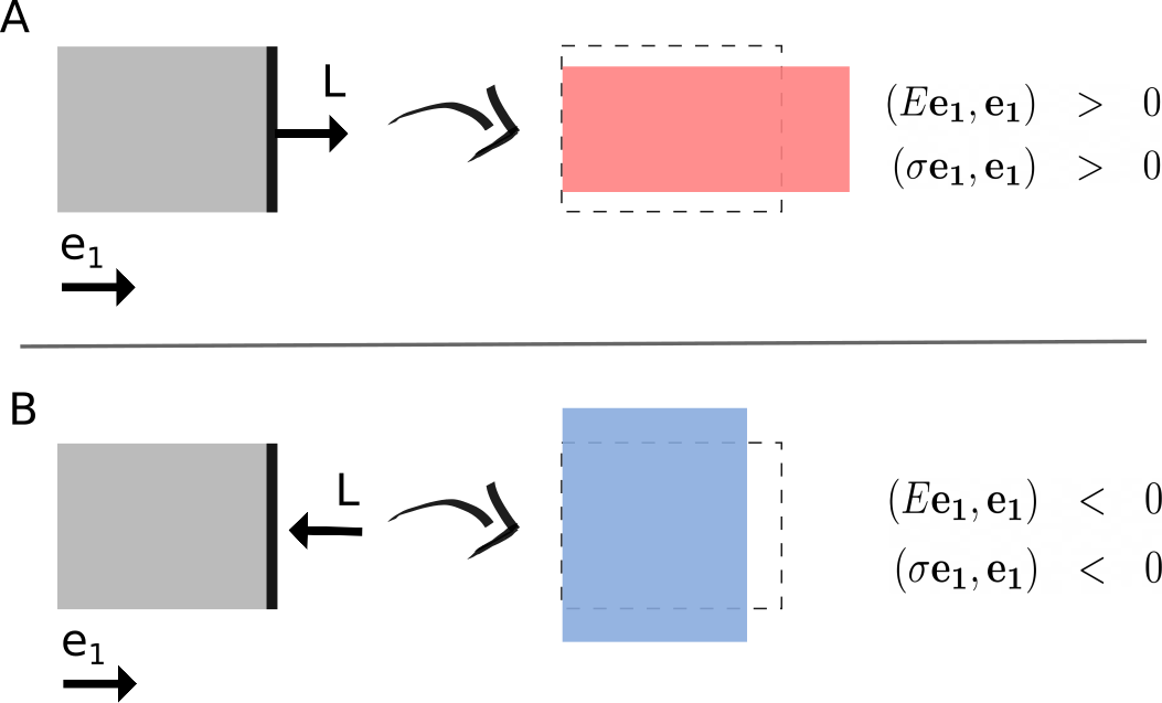
Concepts of strain, stress and load. For a simplified two-dimensional case considering a rectangular domain, we can apply a load \(\mathbf{L}\), which causes the domains to be stretched (A) or compressed (B) in the \(\mathbf{e_1}\) direction. The externally applied load causes an internal positive/negative strain and stress response, respectively, in the direction given by \(\mathbf{e_1}\)
Strain tensors#
The deformation tensor locally defines the change in displacement in all directions, but not the change in displacement relative to the surroundings. This relative change is instead expressed through the concept of strain. Strain is a unit-less quantity that defines the local deformation at any point, in all directions. Zero strain means no deformation; positive strain implies stretching or expansion, while negative strain implies compression or contraction.
From the deformation tensor, the right Cauchy-Green tensor is defined by
which locally gives us the square of local changes in deformation. It might not be so often reported by itself, but is used to derive other key mechanical quantities.
One of these is the Green-Lagrange strain tensor \(\mathbf{E}\), defined by
which gives us the strain relative to the reference configuration. In matrix form, in the vector space spanned by unit vectors representing the fiber, sheet, and normal directions (\(\mathbf{f}\), \(\mathbf{s}\), and \(\mathbf{n}\)), we can write \(\mathbf{E}\) out as
where the subscripts denote the directions. Here \(E_{xy}\) is equivalent to \((\mathbf{E} \mathbf{x}, \mathbf{y})\); for example
The diagonal elements are called normal components and the off-diagonal shear components.
Stress tensors#
In continuum mechanics, stress extends the concept of force. It expresses the internal resistive force per unit area, at any given point, from all directions. For example, if one deforms a material by stretching it, internal forces work in the opposite direction.
The relationship between stress and strain in a hyperelastic material is, per definition, given by a \emph{strain energy function} \(\psi\) \cite{Holzapfel2000}. More specifically, it is a Helmholtz free-energy function that can be expressed only dependent on factors of \(\mathbf{F}\). Often this is via components of \(\mathbf{E}\); of different invariants dependent on \(\mathbf{C}\); however, if written out explicitly, we can always get back to the deformation tensor \(\mathbf{F}\) itself. For ideal elastic solids, the strain energy is the potential energy converted from the work performed on the solid, which is a completely reversible process \cite{Taber2020}.
Strain energy functions are often taken to be continuous, strictly positive, and required to be zero in the reference configuration \cite{Holzapfel2000}. Mathematically, this implies that \(\psi (\mathbf{F}) \geq 0\) for all possible \(\mathbf{F}\) and \(\psi(\mathbf{I}) = 0\). They are also usually monotonously increasing, although they might also capture a decreasing fracture region. If \(\psi\) is non-linear, we have a non-linear material, which is indeed the case for cardiac tissue – actually, most biological tissues can be modeled as such \cite{Chagnon2015}. If it also is defined by a time-dependent component, also common for biological tissues \cite{Taber2020}, we have a viscoelastic material - also a much-used approach in the cardiac mechanics’ society.
If we have different stress-strain ratios in different directions, in which case we have an anisotropic material rather than an isotropic material, this is also captured by \(\psi\). The relation between stress and strain gives rise to characteristic stress-strain curves, specific for any given material.
The second Piola-Kirchhoff stress tensor quantifies the stresses in the current configuration relative to the reference configuration. It can be defined based on the strain energy function by
An equilibrium solution, in which all forces are balanced, can be found solving for
where we assume no acceleration at the center of mass \cite{Taber2020}. In cases where external loads are applied, directly or implicitly through boundary conditions, this also becomes a part of the equation. In the work presented in this thesis, we will often use numerical methods to find the displacement field \(\mathbf{u}\) based on this equation.
The Cauchy stress tensor \(\sigma\) quantifies the stresses in the current configuration relative to the area in the \emph{current} configuration. It is related to \(\mathbf{P}\) by
In matrix form, in the vector space spanned by unit vectors for the fiber, sheet, and normal directions, we can write \(\mathbf{\sigma}\) out as
Here the diagonal components represent the normal stresses and the off-diagonal components the shear stresses. As for \(\mathbf{E}\), the components, we have the equality \(\sigma_{xy} = (\mathbf{\sigma} \mathbf{x}, \mathbf{y})\), for example