Meshes and geometries#
The EMI framework, in which we have an explicit geometrical representation, can be used to differentiate between processes taking place inside of the cells and in the matrix surroudning the. The core idea is that what happens inside the cells is fundamentally different from what happens outside of the cells; and by averaging these out we are missing out interactions taking place on a microscale level.
The geometries represent a fundamental part of the EMI model. In this section, we’ll go through how to read in the meshes which already exist. We will also, towards the end, provide some information about how to generate your own meshes.
We will use the code from the repository emimechanicalmodel, which is based on FEniCS. We can import all libraries we need as following:
import fenics as f
import emimechanicalmodel as emi_m
You don’t really need to know much FEniCS in advance to run the code - we will guide you through what you need to know.
Reading in one mesh file#
We can start by reading in the mesh and subdomain information:
mesh_file = "tile_connected_10p0.h5"
mesh, volumes = emi_m.load_mesh(mesh_file)
Mesh and subdomains loaded successfully.
Number of nodes: 335, number of elements: 1364
Here, the mesh object gives us a tetrahedral representation of our geometry (all nodes and edges) and volumes is a so-called MeshFunction which tells us which elements (tetrahedra) belongs to the intracellular space, and which elements belongs to the extracellular space. We can actually print the meshfunction’s “array” representation to see the data:
print("Subdomain data length: ", len(volumes.array()[:]))
print("Subdomain data: ", volumes.array()[:])
Subdomain data length:  1364
Subdomain data:  [1 1 1 ... 0 0 0]
Here, all the ones represent the cell (the intracellular subdomain) and all the zeros the matrix (the extracellular subdomain).
We can save the volumes object to a pvd file:
f.File("subdomains.pvd") << volumes
In the code you are running the notebook from, you should now have a file called “subdomains.pvd”, as well as a file called “subdomains000000.vtu”, which belong together. You can open either of these in Paraview, and inspect the output. Through Paraview we can visualize the subdomains and the mesh representation, which for our sample mesh can look like this:
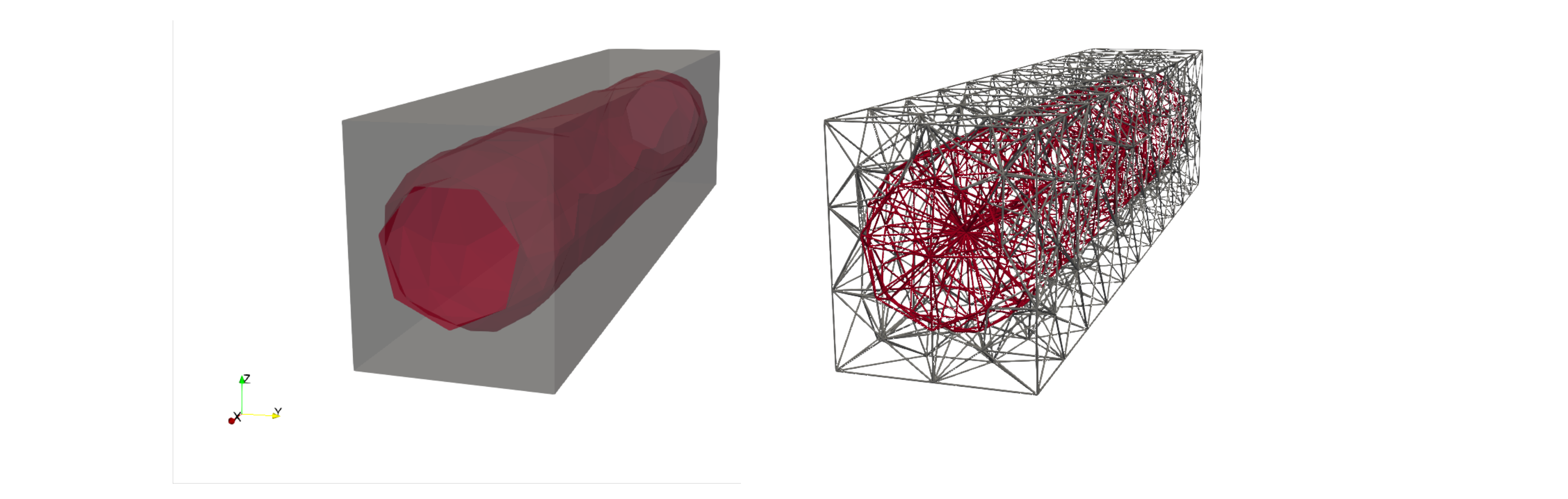
We will denote the intracellular subdomain, i.e., the cell, by \(\Omega_i\), and the extracellular subdomain, i.e., the matrix, by \(\Omega_e\).
Other mesh files#
A number of pre-generated meshes (geometries) are available here.
There are some logical pattern her:
The meshes with an infix “connected” are connected in the longitudinal direction, as opposed to the meshes without this infix, which are not connected from cell to cell.
The infixes “10p0”, “5p0”, etc. indicate the resolution (maximum size of any element in the mesh), generated by the command -clmax in gmsh.
The patterns “_m_n_k” indicate how many cells for multicellular domains; in length, width, and height.
For the multicellular meshes, each cell have their own unique identity number. For e.g. 4 cells, this will be numbers 1, 2, 3, and 4. These will be read in as volumes, and if you open the corresponding meshes in Paraview each cell will be visualized by a different color.
Generating your own meshes.#
The geo files are the fundamental Gmsh files, also available here, that all the meshes are generated by. You can open these in Gmsh (I used version 4.9.5). From a geo file you can generate the mesh for one cell.
The tiling to multicellular domains can next, based on the corresponding .msh files, be performed using the software tieler (as per October 31st, 2022, using the branch “foo”).