Active contraction

The EMI model is based on a core idea that what happens inside the cells is fundamentally different from what happens outside of the cells. In traditional tissue-level models these are averaged out, which is necessesary for many purposes in terms of having a tractable code running in feasible time. For a handful of cells, however, it is quite feasible to take these differences into account.

One of the core principles in the mechanical EMI model is that the cells contract - and the matrix does not. We assume continuity of displacement across the membrane, so the matrix will move with the cells, yet restrict the movement somewhat, especially if it is stiff.

We will use the code from the main repository emimechanicalmodel, which is based on FEniCS. We can import all libraries we need in this demo as follows:

import numpy as np
import matplotlib.pyplot as plt

import fenics as f
import emimechanicalmodel as emi_m

f.set_log_level(30)        # less verbatim output from the Newton solver compared to default

You don’t really need to know much FEniCS in advance to run the code - we will guide you through what you need to know.

Geometries and meshes

We can start by reading in the mesh and subdomain information:

mesh_file = "tile_connected_10p0.h5"
mesh, volumes = emi_m.load_mesh(mesh_file)

Mesh and subdomains loaded successfully.
Number of nodes: 335, number of elements: 1364

Fundamental equations

When we solve the mechanical problem, we want to find a displacement field \(\mathbf{u}\) which gives us an equilibrium of stresses. We are, essentially, solving for a three-dimensional version of Newton’s third law, expressed by Piola-Kirchhoff stress tensor \(\mathbf{P}\):

\[\nabla \cdot \mathbf{P} = 0\]

We allow for free contraction on all sides, such that all forces we deal with are generated by the cell itself. In addition, we need to account for stiffness of each subdomain. The stiffer either is, the harder it will be for the cell to contract. We won’t go into all the details of the derivation here, but in short, we can express \(\mathbf{P}\) as an equilibrium between active and passive forces. There are different ways of implement both, which will be covered in subsequent sections of this book. For now, let’s focus on how to make the model run at all.

Active transient

We will use the force calculated from the Rice model to calculate \(T_{active} (t)\) (using the active stress approach) or \(\gamma\) (using the active strain approach). Note that this is weakly coupled; we are not giving the local strain (which can be translated to the change in the sarcomere length) back to the Rice model. Physiologically this would have made most sense, but this is a non-trivial task – that no-one so far has been able to do for the EMI model!

We have, for convenience, precalculated the force transient which we will read in for now. Later on, we’ll play with some of the parameters to get different active tension transients based on changes in calcium and myofilament dynamics. We can read in, and plot, the pre-calculated values as follows:

time = np.linspace(0, 500, 125)       # 500 ms with 125 steps

active_precomputed = emi_m.compute_active_component(time)

plt.plot(time, active_precomputed)
plt.xlabel("Time (ms)")
plt.ylabel("Active force (kPa); unscaled")
plt.show()

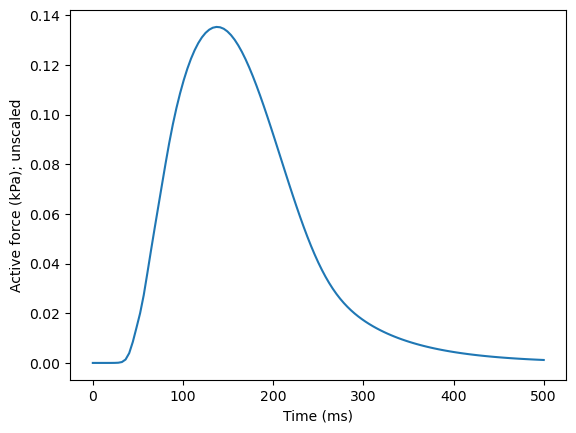
This is meant to resemble half of a single beat (up t0 500 ms, out of 1000). Note that this is a normalized beat, which needs to be scaled up to resemble contraction in a physiologically relevant range. Doubling the magnitude gives reasonable strain values (about 20 % shortening of the cell):

active_precomputed *= 2

This is a scaling parameter that, depepnding on your application, might be useful to experiment with.

Running the EMI model

With the theory explained, let’s move on to the actual coding! From the emimechanicalmodel library, we can make an instance of the EMI model which is based on all the equations above - predefined for us. You hence won’t need to worry about getting any of the equations right; your main task will be to adjust the different parameters.

We can create one instance like this:

emimodel = emi_m.EMIModel(
            mesh,
            volumes,
            experiment="contraction",
        )

Domain length=102.0, width=20.0, height=24.0

The ‘mesh’ and ‘volumes’ parameters are given as explained above, and always needs to be provided. The same goes for the ‘experiment’ parameter, which specifies what kind of deformation to perform. In addition to “contraction”, we can do stretch and shear experiments, which will be demonstrated in the next chapter.

Running a forward simulation

Let’s use the active values from above. We can update the active contraction in a for loop, like this, and solve the system in every iteration.

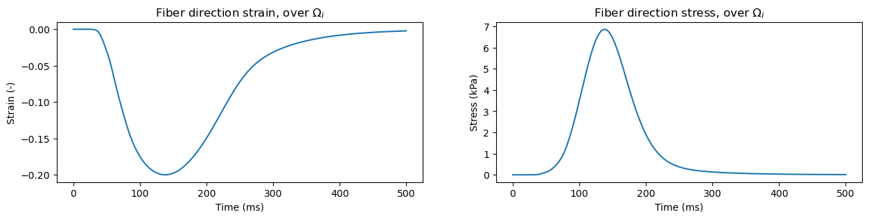
We will track two variables over contraction: The average intracellular strain in the fiber direction, and the intracellular stress in the fiber direction. Mathematically, we are tracking the values

(13)\[\begin{equation} \overline{E_{ff}} = \frac{\int_{\Omega_i} \mathbf{f} \cdot (\mathbf{E} \mathbf{f}) \mathrm{d}\mathbf{X}}{\int_{\Omega i} \mathrm{d}\mathbf{X}} \qquad \text{and} \qquad \overline{\sigma_{ff}} = \frac{\int_{\Omega_i} \mathbf{f} \cdot (\mathbf{\sigma} \mathbf{f}) \mathrm{d}\mathbf{X}}{\int_{\Omega i} \mathrm{d}\mathbf{X}} \label{eq:cm_stress} \end{equation}\]

and while it would certainly be possible to perform these integrals “manually” by writing out the Fenics code for each, this is already implemented so we will simply do this using in-built functions.

fiber_dir_strain_i = np.zeros_like(active_precomputed)
fiber_dir_stress_i = np.zeros_like(active_precomputed) 
subdomain_id = 1         # intracellular subdomain

# then run the simulation
for step, a_str in enumerate(active_precomputed):    
    if (step-1) % 10 == 0:
        print(f"Simulating {step - 1} / {len(active_precomputed)}" + \
              f" with active tension parameter {a_str:.5f}")
    
    emimodel.update_active_fn(a_str)
    emimodel.solve()
    
    fiber_dir_strain_i[step] = \
        emimodel.evaluate_subdomain_strain_fibre_dir(subdomain_id)
    fiber_dir_stress_i[step] = \
        emimodel.evaluate_subdomain_stress_fibre_dir(subdomain_id)

Simulating 0 / 125 with active tension parameter 0.00000

Simulating 10 / 125 with active tension parameter 0.01696

Simulating 20 / 125 with active tension parameter 0.17706

Simulating 30 / 125 with active tension parameter 0.26582

Simulating 40 / 125 with active tension parameter 0.25052

Simulating 50 / 125 with active tension parameter 0.17125

Simulating 60 / 125 with active tension parameter 0.08736

Simulating 70 / 125 with active tension parameter 0.04239

Simulating 80 / 125 with active tension parameter 0.02363

Simulating 90 / 125 with active tension parameter 0.01368

Simulating 100 / 125 with active tension parameter 0.00800

Simulating 110 / 125 with active tension parameter 0.00471

Simulating 120 / 125 with active tension parameter 0.00278

We can next plot these, let’s do them in two separate subplots as they have different units:

fig, axes = plt.subplots(1, 2, figsize=(15, 3))

axes[0].plot(time, fiber_dir_strain_i)
axes[1].plot(time, fiber_dir_stress_i)

axes[0].set_xlabel("Time (ms)")
axes[1].set_xlabel("Time (ms)")
axes[0].set_ylabel("Strain (-)")
axes[1].set_ylabel("Stress (kPa)")

axes[0].set_title(r"Fiber direction strain, over $\Omega_i$")
axes[1].set_title(r"Fiber direction stress, over $\Omega_i$")

plt.show()

In similar manners we can track stresses and strain values in the extracellular subdomain, identified with the number \(0\). We also have in-built functions for tracking sheet and normal direction values, using functions evaluate_subdomain_strain_sheet_dir, evaluate_subdomain_strain_normal_dir, evaluate_subdomain_stress_sheet_dir, and evaluate_subdomain_stress_normal_dir.