Stretch and shear experiments

Stretch and shear experiments#

When we solve the mechanical model, we are solving for an equilibrium of stresses. Here, both active and passive tension plays in, as well as boundary conditions. The passive tension is determined by a strain energy function. The matematical definition will determine the overall behavior – e.g. linear, exponential – together with numerical parameters determining the stiffness of the material for different deformation modes. These parameters are explicitly called material parameters, and determining these for cardiac tissue is a matter of current interest in the cardiac mechanics community.

The strain energy function is usually found by performing stretch and shear experiments of tissue samples (of cardiac tissue), often taken to be cubes. Cardiac tissue is known to be fully orthotropic, i.e., it has different stiffness properties along all three perpendicular axes.

As in the previous chapter, let’s start by importing all libraries we need in this demo:

import numpy as np
import matplotlib.pyplot as plt

import fenics as f
import emimechanicalmodel as emi_m

f.set_log_level(30)        # less verbatim output from the Newton solver compared to default

Next, we can start by reading in the mesh and subdomain information:

mesh_file = "tile_connected_10p0.h5"
mesh, volumes = emi_m.load_mesh(mesh_file)

Mesh and subdomains loaded successfully.
Number of nodes: 335, number of elements: 1364

Fundamental equations#

When we solve the mechanical problem, we want to find a displacement field \(\mathbf{u}\) which gives us an equilibrium of stresses. We are, essentially, solving for a three-dimensional version of Newton’s third law, expressed by Piola-Kirchhoff stress tensor \(\mathbf{P}\):

\[\nabla \cdot \mathbf{P} = 0\]

In this section, we won’t include any active contraction. Instead, we’ll solve for an equilibrium given by the passive properties of the material subject to boundary conditions which will give us the stretching and shearing deformation modes of interest. Here, \(\mathbf{P}\) will depend on the deformation tensor \(\mathbf{F}\) and a given strain energy \(\Psi\):

\[ P = \frac{\partial \Psi (F)}{\partial F}\]

The two core ideas in the EMI model are that both \(\psi_{passive}\) and \(\psi_{active}\) are defined differently for each subdomain. For \(\psi\) as given above, we can separate it into two separate contributions:

\[\begin{split} \Psi (F) = \begin{cases} \Psi_{i} (F) \qquad x \in \Omega_i \\ \Psi_{e} (F) \qquad x \in \Omega_e \end{cases} \end{split}\]

This is, as you might notice, not defined at the membrane itself, i.e., the surface separating the two subdomains. That is, however, not so important; you might think of it as that we assume, for simplicity, that the membrane has zero stiffness (which is not exactly right, but it’s a valid simplification).

Deformation modes of interest#

There are, in general, nine different deformation modes of interest used to determine the material parameters of cardiac tissue – three for stretching the material, and six for shearing the material in a diagonal manner.

A: 25 % shear deformation of the fiber-sheet shear deformation mode \(FS\). B: All nine deformation modes of interest. The white arrows display the direction we move a surface in, while the opposite surface remains fixed. The pink arrows display the normals of the same surfaces.

There are two ways to perform stretching (and shearing) experiments. They are two sides of the same coin; applying one approach we can calculate the result in the other, and vice versa. One way, and prehaps the most normal one, is to apply a load on one surface while fixing the opposite one. That will result in that the domain moves on one side, from which one can calculate a resulting displacement. For the EMI model, however, since we have different intra- and extracellular stiffness properties this would result in a spatially varying displacement, dependent on the cellular geometry.

The other one, which we will use in our model, is to prescribe a displacement. For a given displacement (i.e., a given stretch value) we can, based on the resulting stress values, calculate the resulting load on a given surface. We will prescribe the stretch using a constant value; and the resulting load will then be a spatially varying variable. When we report on the load values, this is actually calculated as a surface integral over the given surface, normalized by the surface area.

Running the EMI model#

With the theory explained, let’s get the model running! From the emimechanicalmodel library, we can make an instance of the EMI model which is based on all the equations above. The instances will be defined differently for each stretching and shearing mode.

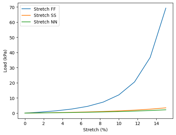
Stretching experiments#

Let’s first perform the three stretching experiments – in the fiber, sheet, and normal directions. As we stretch the domain in different direcitons, we’ll track the (averaged) normal load values.

deformation_modes = ["stretch_ff", "stretch_ss", "stretch_nn"]
labels = ["Stretch FF", "Stretch SS", "Stretch NN"]

stretch_values = np.linspace(0, 0.15, 10)           # up to 15 % in 10 steps

for deformation_mode, label in zip(deformation_modes, labels):

    emimodel = emi_m.EMIModel(
            mesh,
            volumes,
            experiment=deformation_mode,
        )

    load_values = np.zeros_like(stretch_values)
    
    # then run the simulation
    for step, stretch_value in enumerate(stretch_values):
        emimodel.assign_stretch(stretch_value)
        emimodel.solve()
        
        load_values[step] = emimodel.evaluate_normal_load()
    
    plt.plot(100*stretch_values, load_values, label=label)

plt.xlabel("Stretch (%)")
plt.ylabel("Load (kPa)")

plt.legend()
plt.show()

Domain length=102.0, width=20.0, height=24.0

0.0
load:  3.286738961392422e-16
0.016666666666666666

load:  0.6661736926140899
0.03333333333333333

load:  1.5131466777821316
0.05

load:  2.6893072404992244
0.06666666666666667

load:  4.449028545778154
0.08333333333333333

load:  7.258046605211915
0.1

load:  12.0140186753059
0.11666666666666667

load:  20.53642287176041
0.13333333333333333

load:  36.70760895075521
0.15

load:  69.26606753235922
Domain length=102.0, width=20.0, height=24.0

0.0
load:  2.326665247791059e-16
0.016666666666666666

load:  0.15583643713551323
0.03333333333333333

load:  0.3290155762119321
0.05

load:  0.5321545559200578
0.06666666666666667

load:  0.7773602835814413
0.08333333333333333

load:  1.080400317077704
0.1

load:  1.4632414093585715
0.11666666666666667

load:  1.9567206021783885
0.13333333333333333

load:  2.6043806398488885
0.15

load:  3.468243665661275
Domain length=102.0, width=20.0, height=24.0

0.0
load:  2.22520192647767e-16
0.016666666666666666

load:  0.11588786541173554
0.03333333333333333

load:  0.24278649610556433
0.05

load:  0.3892644264483312
0.06666666666666667
load:  0.562521663725653
0.08333333333333333

load:  0.7700019008332939
0.1

load:  1.0209886505821553
0.11666666666666667

load:  1.3278966608896488
0.13333333333333333

load:  1.7075170655058245
0.15

load:  2.182536257762294

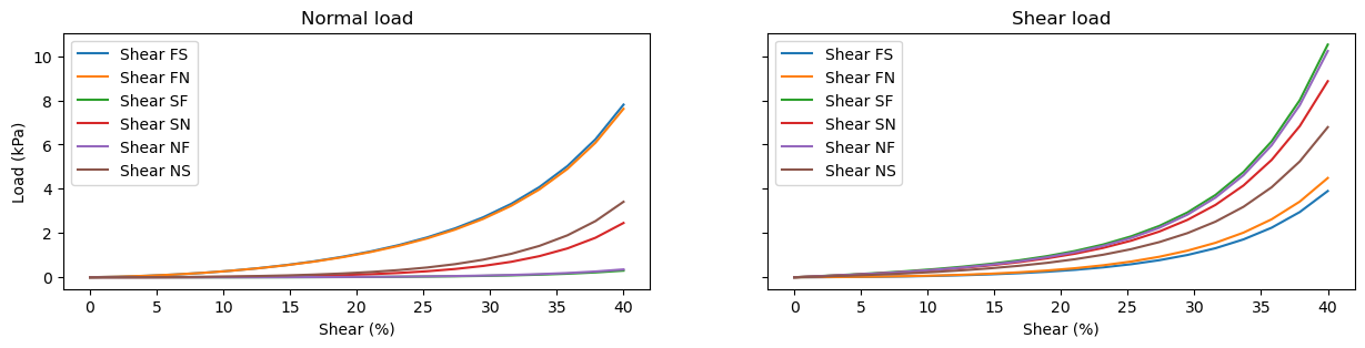
../_images/b393dbfa291c6e7b4d7f391ea42cbd1668c872482d32adb50dd0320b33de5f13.png

Shearing experiments#

In a similar manner, we can perform shear experiments simply by specifying what kind of experiments we want to perform. For these, we’ll track both normal and shear load values (which were coinciding for the stretching experiments):

deformation_modes = ["shear_fs", "shear_fn", "shear_sf", "shear_sn", "shear_nf", "shear_ns"]
labels = ["Shear FS", "Shear FN", "Shear SF", "Shear SN", "Shear NF", "Shear NS"]

stretch_values = np.linspace(0, 0.4, 20)           # up to 40 % in 20 steps

fig, axes = plt.subplots(1, 2, figsize=(15, 3), sharey=True, sharex=True)

for deformation_mode, label in zip(deformation_modes, labels):

    emimodel = emi_m.EMIModel(
            mesh,
            volumes,
            experiment=deformation_mode,
        )

    normal_load_values = np.zeros_like(stretch_values)
    shear_load_values = np.zeros_like(stretch_values)
    
    # then run the simulation
    for step, stretch_value in enumerate(stretch_values):
        emimodel.assign_stretch(stretch_value)
        emimodel.solve()
        
        normal_load_values[step] = emimodel.evaluate_normal_load()
        shear_load_values[step] = emimodel.evaluate_shear_load()
    
    axes[0].plot(100*stretch_values, normal_load_values, label=label)
    axes[1].plot(100*stretch_values, shear_load_values, label=label)

axes[0].set_xlabel("Shear (%)")
axes[1].set_xlabel("Shear (%)")
axes[0].set_ylabel("Load (kPa)")

axes[0].set_title("Normal load")
axes[1].set_title("Shear load")

axes[0].legend()
axes[1].legend()

plt.legend()
plt.show()

Domain length=102.0, width=20.0, height=24.0

0.0
load:  3.286738961392422e-16
HER!
Calling FFC just-in-time (JIT) compiler, this may take some time.

Calling FFC just-in-time (JIT) compiler, this may take some time.

0.021052631578947368

load:  0.025597860617822595
HER!
0.042105263157894736

load:  0.06593762016372985
HER!
0.06315789473684211

load:  0.12304696663714472
HER!
0.08421052631578947

load:  0.19882535313591668
HER!
0.10526315789473684

load:  0.29461581562338895
HER!
0.12631578947368421

load:  0.41240138197674087
HER!
0.14736842105263157

load:  0.5552111169322019
HER!
0.16842105263157894

load:  0.7263103820824345
HER!
0.18947368421052632

load:  0.9298950344014278
HER!
0.21052631578947367

load:  1.1715039908689289
HER!
0.23157894736842105

load:  1.4587140701915935
HER!
0.25263157894736843

load:  1.8018073816292792
HER!
0.2736842105263158

load:  2.2133635989718763
HER!
0.29473684210526313

load:  2.71174792581233
HER!
0.3157894736842105

load:  3.3212751511796967
HER!
0.3368421052631579

load:  4.077473600748668
HER!
0.35789473684210527

load:  5.027702457952311
HER!
0.37894736842105264

load:  6.239738833910146
HER!
0.4

load:  7.8078300301534815
HER!
Domain length=102.0, width=20.0, height=24.0

0.0
load:  3.286738961392422e-16
Calling FFC just-in-time (JIT) compiler, this may take some time.

Calling FFC just-in-time (JIT) compiler, this may take some time.

0.021052631578947368

load:  0.026385994871219884
0.042105263157894736

load:  0.06719801700586903
0.06315789473684211

load:  0.12430771156073395
0.08421052631578947

load:  0.19899664483993212
0.10526315789473684

load:  0.29285445331316934
0.12631578947368421

load:  0.4078521003770479
0.14736842105263157

load:  0.5464331100361199
0.16842105263157894

load:  0.712130471390473
0.18947368421052632

load:  0.9093486894027599
0.21052631578947367

load:  1.1437080490957534
0.23157894736842105

load:  1.423146624219708
0.25263157894736843

load:  1.7564738604615069
0.2736842105263158

load:  2.1558274266870057
0.29473684210526313

load:  2.6391848540936995
0.3157894736842105

load:  3.2326296867608213
0.3368421052631579

load:  3.9696295617450637
0.35789473684210527

load:  4.897634370057015
0.37894736842105264

load:  6.083739696628691
0.4

load:  7.619468612776885
Domain length=102.0, width=20.0, height=24.0

0.0
load:  2.326665247791059e-16
Calling FFC just-in-time (JIT) compiler, this may take some time.

Calling FFC just-in-time (JIT) compiler, this may take some time.

0.021052631578947368

load:  -0.0006075608568460203
0.042105263157894736

load:  -0.001006837768616472
0.06315789473684211

load:  -0.0011366389336537055
0.08421052631578947

load:  -0.0009003916893882572
0.10526315789473684

load:  -0.00018906112504850426
0.12631578947368421

load:  0.0011038010098758954
0.14736842105263157

load:  0.0031199281347586622
0.16842105263157894

load:  0.00602437282405834
0.18947368421052632

load:  0.010042334118122874
0.21052631578947367

load:  0.015484455967821945
0.23157894736842105

load:  0.02278172676722061
0.25263157894736843

load:  0.03252289844869625
0.2736842105263158

load:  0.04554007677447414
0.29473684210526313

load:  0.06296671884956359
0.3157894736842105

load:  0.08640405903465527
0.3368421052631579

load:  0.11808512448084414
0.35789473684210527

load:  0.1611774351081857
0.37894736842105264

load:  0.22020627790886707
0.4

load:  0.3015883235045396
Domain length=102.0, width=20.0, height=24.0

0.0
load:  2.326665247791059e-16
Calling FFC just-in-time (JIT) compiler, this may take some time.

Calling FFC just-in-time (JIT) compiler, this may take some time.

0.021052631578947368

load:  0.00010877558169180695
0.042105263157894736

load:  0.001253889046463871
0.06315789473684211

load:  0.0038977945370713405
0.08421052631578947

load:  0.008677634352956806
0.10526315789473684

load:  0.016359618304923686
0.12631578947368421

load:  0.02785322225514925
0.14736842105263157

load:  0.044281678136999826
0.16842105263157894

load:  0.0671181214548395
0.18947368421052632

load:  0.09826401148091823
0.21052631578947367

load:  0.14033082163239546
0.23157894736842105

load:  0.19690140071546924
0.25263157894736843

load:  0.2728802602034629
0.2736842105263158

load:  0.37511839813161035
0.29473684210526313

load:  0.5131278841120377
0.3157894736842105

load:  0.7002338757882456
0.3368421052631579

load:  0.9552849535782185
0.35789473684210527

load:  1.3050099712831507
0.37894736842105264

load:  1.7873814814719924
0.4

load:  2.4569142247770763
Domain length=102.0, width=20.0, height=24.0

0.0
load:  2.22520192647767e-16
Calling FFC just-in-time (JIT) compiler, this may take some time.

Calling FFC just-in-time (JIT) compiler, this may take some time.

0.021052631578947368

load:  -0.00037644122772738945
0.042105263157894736

load:  -0.0005293045529008245
0.06315789473684211

load:  -0.00039830382685725137
0.08421052631578947

load:  0.00011523827247665025
0.10526315789473684

load:  0.0011418065215113575
0.12631578947368421

load:  0.002834712281931535
0.14736842105263157

load:  0.005373713950186238
0.16842105263157894

load:  0.008965423683690773
0.18947368421052632

load:  0.013889184175222963
0.21052631578947367

load:  0.020509634239670192
0.23157894736842105

load:  0.02932826719141513
0.25263157894736843

load:  0.041028413141387804
0.2736842105263158

load:  0.0565656134309104
0.29473684210526313

load:  0.07726822093558526
0.3157894736842105

load:  0.10498470351428231
0.3368421052631579

load:  0.14228454090545462
0.35789473684210527

load:  0.19277634196683063
0.37894736842105264

load:  0.261547049865692
0.4

load:  0.3557916846056509
Domain length=102.0, width=20.0, height=24.0

0.0
load:  2.22520192647767e-16
Calling FFC just-in-time (JIT) compiler, this may take some time.

Calling FFC just-in-time (JIT) compiler, this may take some time.

0.021052631578947368

load:  0.0020544793950024644
0.042105263157894736

load:  0.006065783867752012
0.06315789473684211

load:  0.012629082189281386
0.08421052631578947

load:  0.02260233943885427
0.10526315789473684

load:  0.03707899620991505
0.12631578947368421

load:  0.05741868989025416
0.14736842105263157

load:  0.08531830222430463
0.16842105263157894

load:  0.12294055937755377
0.18947368421052632

load:  0.17309688513791302
0.21052631578947367

load:  0.23946890759619546
0.23157894736842105

load:  0.32698705180961557
0.25263157894736843

load:  0.4422146454821162
0.2736842105263158

load:  0.5941502822108048
0.29473684210526313

load:  0.7951350170357359
0.3157894736842105

load:  1.0620980906814066
0.3368421052631579

load:  1.4184457428757569
0.35789473684210527

load:  1.8964751495906051
0.37894736842105264

load:  2.541197104031234
0.4

load:  3.415657591447898

../_images/0a3a049aad775e77137873abe2039718ac3d4b25e4e2ea7c59fc0a7eb29cd320.png

In the second paper we used all of these experiments for parametrization of the model; see methods section for more details.